Multi-element geological data clustering
There has been some renewed discussion recently around the topic of domaining: the art of selecting which points should or should not be considered part of a domain.In this regard domaining can be considered a form of clustering. In this post we will explain a novel technique we have developed over recent months to help shed more light on correlations, ie. clusters, in data that will hopefully improve understanding of domains and even geological formations. But first a quick recap
In many deposits the outline (shell) of an orebody is created by interpolation of the element of interest. To this end, geostatistics relies on Kriging in its many forms. For those not quite familiar with Kriging interpolation, in a nutshell it is a weighted average using nearby points. The weighting is done based on the distance of the nearby points if they are considered correlated. The latter is typically established by variography where the furthest distance between points still considered to be correlated is a crucial measure. This explanation might upset some geostatisticians, but it is only meant to give a summary without going into details.
Although Kriging has a number of shortcomings, as greatly described by Stephen Henley and some of his peers, S. Henley with D.F. Watson, Possible alternatives to geostatistics: APCOM 1998, London,p.337-354. One of the shortcomings is that Kriging is generally only applied on a single element.
Methods do exist using multiple elements, but are often cumbersome and only useful for the initiated. Therefore, that analysis is generally omitted. And even so, it is typically not used across a whole range of elements at once.
A new approach: multi-dimensional similarity clustering
One of the key assumptions in Kriging is the relationship between distance and correlation of data. It follows from an intuitive understanding that samples close together will exhibit the same properties. In other words, if you find a high-grade sample, you expect to find more in its vicinity. Interestingly, this concept is exactly what Machine Learning (ML) is based on. It looks at patterns of similarities between samples of data such as images.
In GEOREKA, we thought we could apply this ML principle to geological samples. We asked ourselves how we could generate similarity patterns between points in drilling data. That is when we realized that typical clustering is done between samples in 3D space. Again, points close to each other can be thought of as part of a cluster. But what if we do not just consider the X, Y and Z coordinates, but all elements, such as As, Au, Ag, Mo, Pb, Zn etc. Combining all elements, with XYZ coordinates then forms a so-called higher-dimensional space, or in ML terms, hyperspace. Using a similarity pattern system, we could then try to group points together that show a similarity across all elements comparable with normal clustering analysis. And that is roughly what we did.
Similarity clustering in practice
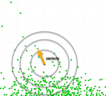
Our approach organizes points into a higher-dimensional cluster and the user provides a reference point within that cluster. The system then estimates a similarity measure between that reference and every other point. The resulting values are then scaled between 0 and 100, where 100 means ‘perfect similarity’ and typically corresponds only to the reference point itself.
Displaying the points back in 3D together with the original data then can be used to highlight regions of high or low similarities.
Some initial results
Parker challenge sub-domains?
One of the data set we applied our algorithm on was the Parker Challenge data (unfortunately, after the challenge was closed): https://www.ausimm.com/conferences-and-events/mineral-resource-estimation/the-parker-challenge/
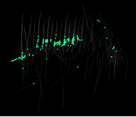
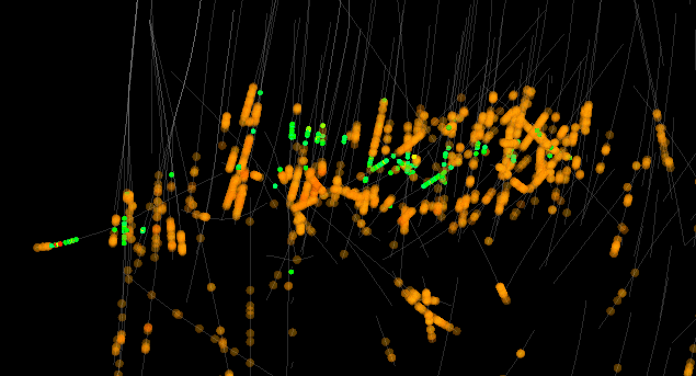
On first glance, the copper grades seemed fairly easy to understand.
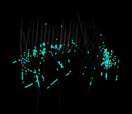
The Au grades showed a slightly different picture, but a large part of the Au seemed to follow the same Cu trend.
Next, we selected two reference points. The first was roughly at the center of the higher-grade copper region. The second was in a ‘nearby’ region approximately 390m away for a high-grade Au sample. We then applied our analysis using each reference point separately. In both cases we used the same attributes (Au, Cu, As and Mo and XYZ) to create our similarity measurements.
The copper similarities exhibited results as expected from the high copper grades and followed a similar trend.
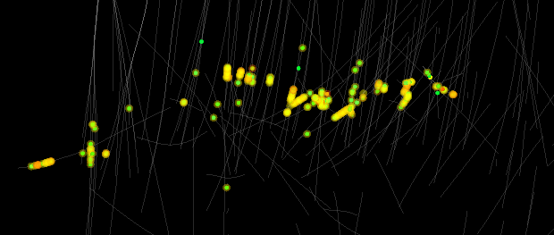
However, the gold grades similarity values did not follow the expected pattern. Instead, the Au clustered data showed up like a halo around the high copper grades.
Even more striking was the fac that the Copper cluster ended up on the other end of the spectrum when looking at the frequency plot of the estimated similarity values for the Au reference point.
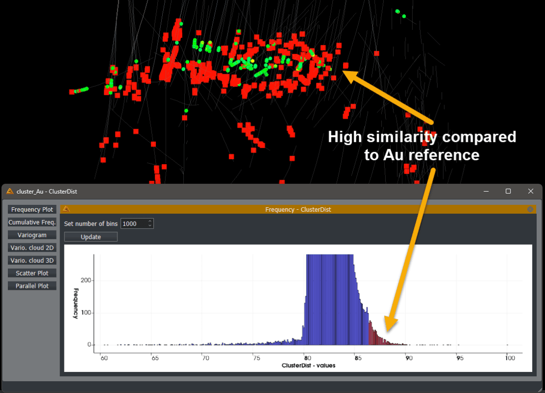
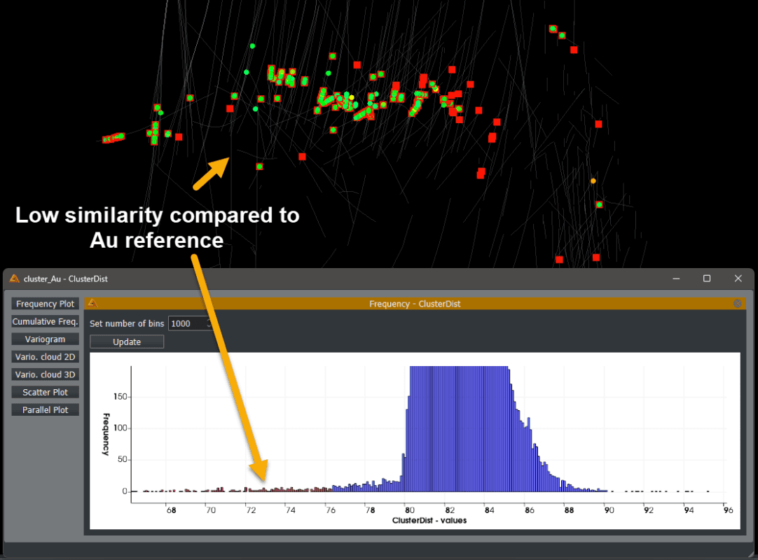
The most reasonable explanation seems to be due to a correlation between the Au and As and / or Mo for our reference point. From our analysis it seems there are two groups of gold ‘clusters’, one highly correlated with As / Mo creating that halo effect, the other one not at all and seems to follow the Cu trend. The question then becomes if they should be separate groups for geostatistical analysis or not? Maybe at a geomettalurgy level, or even at resource level?
A full analysis and explanation can be viewed in our YouTube video: https://youtu.be/UYziWx4g08Y
Geophyisics and lithology
In another example we analyzed geological data with geophysics. Based on Conductivity and Gamma we were able to differentiate not only ore from waste, but even a significant third group. Unfortunately, at the time of writing we are not allowed to share any part of the data. Suffice it to say for now, the tool appears to have the ability to ‘predict’ the lithological unit based on a single reference drillhole just from geophysics.
Caveats – further work
As mentioned here and in other places, the tool is a work-in-progress. It appears to highlight patterns in the data that were not obvious from single-element analysis.
The tool works by manually selecting a reference point. The choice of that selection can greatly influence the ability to cluster points and has been demonstrated with the Parker data. How sensitive it is to the reference points and the resulting conclusions that can be drawn from that remain an area of investigation. The tool seems to demonstrate the ability to quickly highlight patterns. What these patterns mean is subject to the data and understanding thereof.
Note that in our work categorical data has not been used at all. The reasons for this are that categorical data is highly subjective, but also not continuous.
