Machine Learning (ML) Demystified
Anywhere on the internet there is talk about AI and Machine Learning. Many have promoted the use of both within the mining industry. Up until now, there has been limited to no significant breakthrough and means the technology is becoming more and more questioned or even receiving negative connotations. This is understandable, but not completely warranted. Partly it is because of the overwhelming number of possible techniques (see next paragraph) and a lack of understanding them. But partly it is due to language issues, where the ML community is using different labels than the geosciences.
In this article we will try to translate ‘ML speak’ and go a bit more into depth about various Machine Learning techniques with its pros and cons to lift some of the mist that surrounds ML. Hopefully this will help to understand better how it can be used as part of geological modelling.
Three main techniques
Within ML there are many variants for training as illustrated by the list mentioned on the Scikit-learn webpage (https://scikit-learn.org/stable/supervised_learning.html#supervised-learning). For our purposes, geological modelling, three main training techniques stand out and will be the ones we will focus on here: Neural Networks (NNs), Support Vector Machines (SVMs) and Gaussian Processes (GPs). Searching the net you’ll find that all three are in turn closely related. The mathematics is beyond the scope of this article, and to some extend even beyond our capabilities to understand in-depth. However, we’ll highlight some of the similarities and differences related to existing modelling techniques to put ML into perspective.
Before we continue to delve into the main three techniques, just a quick word on what we are actually trying to do in Geological modelling. With some abstraction we can distinguish two main goals: classification (modelling categorical data like lithology) and numeric interpolation also called regression (e.g. for assays).
Let’s focus on classification first
In geology, we try to model geological features, like rock type or certain zones in 3D space. Traditionally this is done by defining a boundary between units. A typical approach would connect the boundary points (found down drill logs) between the unit to model, let’s call it unit A. To model unit A the contact points with any other unit would be extracted and connected, either using digitizing or implicit modelling techniques.
Now, let’s return to our ML techniques. Modelling categorical data as described above amounts to a classification between unit A and everything else. Any of the techniques described above is capable of classification of data, but there are important differences.
We’ll start with Gaussian Processes (GPs)
Gaussian Processes (also called Gaussian Process Regression) are very powerful and have a unique capability compared to the other two techniques we mentioned above: not only can it estimate the boundary (the contact) between a unit A and other units, it also produces the variance between known points. The best is to compare it with implicit modelling where a surface is created through all contact points. What happens in between the points is the interesting bit. With implicit modelling we only obtain a single surface, assumed to be the best fit. Gaussian Processes also produce this boundary, but also give a sense of reliability in between the known points… But hold on… does that not seem a little familiar? Do you know about a technique in geological modelling or geostats that is very similar. Let me help you here. Within geostats there is something called Conditional Simulation. A best guess is created using Kriging and uses the variance around that best fit. In conditional simulation we produce estimates, e.g. inside blocks, to create some ‘noise’ around the Kriging estimate to better re-create reality. To this end the Kriging estimate is used with noise added based on the estimated variance. Here, conditional is referring to the condition that we have known points that need to be honoured. In 1D, Kriging with variance would could like the image on the right.
If you search a bit, GPs are at the least very similar to Kriging, possibly with conditional simulation (https://scikit-learn.org/stable/modules/gaussian_process.html#gaussian-process-regression-gpr).
To illustrate, we also give a 1D example for Gaussian Process Regression.
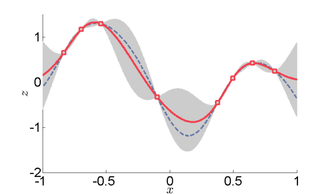
Example of 1D kriging (https://en.wikipedia.org/wiki/Kriging)
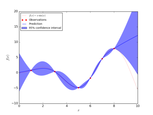
Example of 1D Gaussian Process from popular site Scikit-learn (https://scikit-learn.org/0.17/auto_examples/gaussian_process/plot_gp_regression.html)
If you click the link to the fundamental webpage on Gaussian Processes (http://gaussianprocess.org), notice how on the main webpage Kriging is listed as one of the recommended books.
But, moreover, check the wikipedia page on Kriging itself:
https://en.wikipedia.org/wiki/Kriging
The first line is: “In statistics, originally in geostatistics, kriging or Kriging, also known as Gaussian process regression“…
So, yes, this “Machine Learning technique” is nothing new to geology! It seems to actually be derived from techniques used in the industry for decades!!
OK, well, now you know that you have been doing a form of Machine Learning most of your modelling life. I bet you already will sleep a lot better…
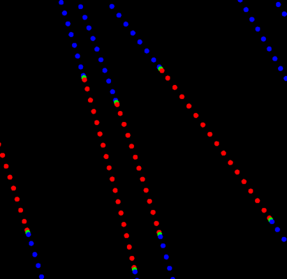
Example showing categorical data being converted into indicator points (inside points: red = +1, boundary: green = 0, outside: blue = -1)
Now, let us focus on Support Vector Machines (SVMs)
Above, we already mentioned implicit modelling as being one of the traditional methods to define a boundary between categorical data. To this end the categorical data is typically converted to numeric data. In this conversion process the unit to model is labelled with positive indicator points, the boundary points with a zero value and all other units are converted to negative values. In most cases the inside values will be converted to +1, the outside values to -1. This might not always be obvious, but is what actually happens inside the software (others might not use indicator values, but positive and negative distance values, but the principle is the same). It means the categorical data is turned into classification data [-1, 0, +1].
In implicit modelling, so-called Radial Basis Functions (RBFs) are fitted through all the points with their values as if the values were on a continuous scale. It has been shown that fitting RBFs in this way is akin to Kriging already in 1996 (https://www.researchgate.net/publication/216837924_Fast_Multidimensional_Interpolations).
The most important part to remember about this is that a radial basis function is used at each point in the data set. Such functions are typically a Gaussian or other smooth function. A single RBF will produce a value that is dependent on the distance from a point in the original data to another point in that data set. Doing this for each point to every other point you end up with many RBFs. This becomes inefficient for points far away, so clever techniques have been developed to make that a lot faster.
The aim is then to fit, in other words learn, the weights of each of these functions (so, one weight per function) to reproduce the original data.
Now compare that to Support Vector Machines (SVMs). In SVMs also Radial Basis Functions (RBFs) are used to get a relation between each point in a data set and every other point in that data set. However, in the case of SVMs the RBF is called a kernel. Similar to fitting RBFs, for each point in the data the kernel is used to calculate a measure related to the distance to every other point. All these values are treated as a (very) long vector associated with that particular point. This means you have a large set of very long vectors. Due to efficient mathematics involving dot products (a dot product of two vectors returns the ‘angle’ between them) points that have high similarity (a small angle) are used to separate the groups of points, others are discarded. Using these vectors a so-called hyperplane can be identified that will separate the +1 points from the -1 points. This hyperplane is guaranteed to be the best fit plane separating the groups (compare it a bit to Least Square fitting). So, although the technique is slightly different to direct fitting of RBFs, the basis is roughly the same. Especially when optimized RBFs are considered that actually filter or group points together (e.g. for fast RBF implementations; https://www.researchgate.net/publication/2931421_Reconstruction_and_Representation_of_3D_Objects_With_Radial_Basis_Functions)
The important difference to remember is that RBFs (without speed improvements) will fit exactly to the known points, most notably the boundary. SVMs on the other hand will produce a boundary that is the best fit between two groups of points. This means its boundary might not always honour the points on the boundary exactly if inside and outside points are not equally far from the boundary. The advantage of SVMs is that they will ‘learn’ really quickly, but also will produce very good estimates in areas where the contact is not very clear or uncertain. Also, in SVMs, a penalty can be applied to wrongfully classifying a number of points. This will control the accuracy of the separation, just like in RBFs we do not always fit exactly through the points to improve the speed (by setting an accuracy value).
To illustrate a bit further, on the right we show examples for separating two groups of points (https://towardsdatascience.com/support-vector-machine-introduction-to-machine-learning-algorithms-934a444fca47). In the top one, shows a number of possible separations, the bottom only shows the optimal separation. It almost becomes like a Kriging estimate (optimal plane) with conditional simulation (other possible planes).
The optimal separation plane, when converted back to 3D is the estimated contact between two unit.
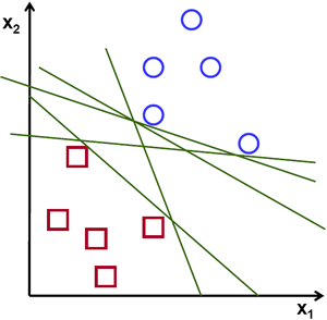
Example of possible separation planes for classification of data using SVMs
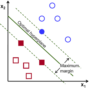
The optimal separation plane for the same data (https://towardsdatascience.com/support-vector-machine-introduction-to-machine-learning-algorithms-934a444fca47)
Finally, we will get to Neural Networks (NNs)
As with SVMs, there are a whole lot of variants of NNs. People might refer to Convolution Networks, Deep Learning and many other things, but essentially they are based on the traditional NNs. One of the attractions that has generated the interest in NNs in the first place, is their ability reproduce any continuos function (https://www.baeldung.com/cs/neural-net-advantages-disadvantages#universal-approximation-theorem-and-its-limitation) under two important assumptions: enough data and using enough nodes. So, let’s explain a bit how NNs work. In its most basic form a NN will have an input layer. This just determines which parameters will be used as input. For geological modelling these would most likely be X, Y and Z. On the output the values from the middle layer (see below) are grouped together (summed) and, based on a threshold, a classification value is computed. For the original data set, the computed value is compared to the known value (just to keep consistent with RBF’s and Kriging etc, these would be the indicator values, as before). Similarities and differences will be used to train the weights in the magic layer (normally called the hidden layer): https://en.wikipedia.org/wiki/Neural_network
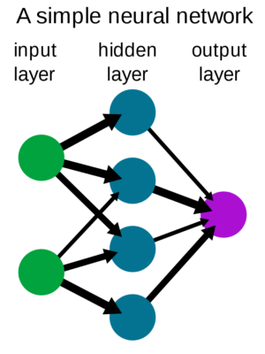
We call this the magic layer here as this is where most of the magic happens. Each so-called node in the magic layer contains a function, traditionally an RBF. Yes, again the Gaussian function is often used here. Each node in the magic layer will take all values from the previous layer (the X, Y, and Z) and produce an output based on the weight associated with its RBF. When the number of nodes is set to the number of points it should theoretically reproduce the exact results for the original points as each node will represent a single point in the data set. The aim is to find / reduce the number of nodes that will still yield accurate results.
NNs start their training by assigning some random weights to the RBFs in the network. Then for a sub-set of the original data the weights are determined that will predict the correct classification by repeatedly feeding points into the network, calculating the output and using the differences with the known values to update the internal weights. The remaining set of points, those not used during training, are used to constrain the network not to only predict the known points, but also unknown points.
As you can see, NNs are a bit more involved to find the right weights. However, when they are found they tend to be very quick in estimating the output at unknown locations. Another important aspect is that due to starting with some random weights, each time a network is trained it might produce slightly different results. This means trained networks are de facto not reproducible. But also, this randomness might mean the network will sometimes not learn at all, or sometimes it might be very quick to learn the right output.
Much work has been put into improving behaviour of NNs to limit the effect of the randomness at the start. Also systems exist that will try to determine the number of nodes in a network by itself.
Deep learning uses the same approach as NNs, but just has multiple magic layers.
If we compare the NNs to SVMs some say the NNs will also find a hyperplane that will separate two classes. However, due to its nature, NNs are not guaranteed to find the optimal plane that has the maximum distance to either group of points. It is more like a single realization from conditional simulation (or Gaussian Processes for that matter). This means sometimes it will be very good, other times not. A very good post comparing NNs with SVMs is given here: https://www.baeldung.com/cs/svm-vs-neural-network
Short summary
In the above we have given a very brief introduction to the various Machine Learning tools out in the world. Hopefully, we have been able to show that they are not so dissimilar from tools already known and used within geological modelling.
One thing we would like to draw your attention to the idea of distance measures. In GPs the Gaussian kernel is used as a measure, in implicit modelling and SVMs, a Gaussian RBF is also the default kernel for non-linear separation. Finally, the Gaussian function is typically used in NNs for the nodes.
This brings it all back to the basic idea that points close to each other will typically be related, whereas points further away are generally less likely to be correlated. That is what all methods have in common. For certain tasks a Gaussian is not always the best, so, depending on the interpolation method, you’ll see alternative RBFs (kernels) being used that better suit the problem.
Some conclusions: No more black boxes?
As we hope to have demonstrated ML does not constitute some magic that will automatically produce better models than what we have been doing in the industry already. We need to realize that the data feeding into any ML technique does not contain any relationships between points. This means none of the ML techniques will understand what geology is or any geological constraints. This leads us to three important conclusions:
- To highlight a single aspect let us concentrate on Anisotropy. ML’s only task is to separate one group from another (when looking at geological modelling). To this end, it could ‘draw a sphere’ around each inside point. This sphere should be so small that it will not contain another point. Within this sphere everything is always inside the unit to model. From an ML point of view that would be a good solution. Understandably, this will not yield a useful geological model. However, in reality it is probably not far off from what really happens if no knowledge is supplied to the data. Spheres that are overlapping / connecting might be merged. As you can see that approach will amount to an isotropic interpolation which generally yields bad results. So, like in our traditional modelling we will (in most cases) need to specify an anisotropy to the data before feeding it into an ML system.
- Secondly, as we briefly mentioned, ML will, just like in implicit modelling, assume a continuous space. It cannot handle discrete changes, like faults. Instead, it will ‘smear’ the output across the fault.
- Thirdly, as with any ‘interpolation’ technique, outside the space of the input points, ML techniques will extrapolate. And just like any other technique extrapolation needs to be handled with a lot of caution (more on this in a separate article). In ML language this often refers to over-fitting when done badly, or good generalisation when done correctly.
Some recommendations
The goal of this article was not to discourage people from using ML techniques. But, like anything, care needs to be taken that they are applied in the proper way. As we highlighted in our conclusions, feeding a ML system with all data we have (even if assuming all data has been cleaned and validated etc.) and expecting amazing results will not happen. This will just lead to a situation where ML will be dismissed as ‘It doesn’t work!’. That would be a real shame as there is some real value. Therefore we decided to provide some recommendations to help getting the most of the exciting ML developments.
1) Understanding basic ML techniques
GPs are very similar to Kriging and Conditional Simulation (CS). The main difference, it seems, is in the assumption that data is normally distributed. In geology we know this is almost never the case. This means instead of using the simple Covariance that is used in GPs we’ll need to use Variography. Integrating Variography with GP tools could be very interesting. Maybe it will then become just Kriging, or maybe it will just allow more people to use ML in their modelling to highlight uncertainty.
NNs take a relatively long time to train. They are really good for generating estimates after being trained (very fast evaluations). Within geology we do not see a lot of use for NNs. Since each geological setting is highly unique, having trained a system for one project (assuming it can be done correctly) it cannot be applied to another project. Furthermore, its random nature also means results will not be reproducible when trained again (unless using sophisticated controls that will guarantee to always find the same results). And finally, it remains a difficult problem to define the NN, i.e. how many nodes are needed, how many layers, etc. For geological modelling, this will make it rather useless as it doesn’t offer any major benefits compared to SVMs and GPs.
Finally, SVMs are a fast way for modelling geological classifications. Its approach means results are reproducible and controlled. It however lacks the ability to model uncertainty directly as with GPs. On the other hand, its similarity to implicit modelling means it can be a near direct substitution.
2) Understanding the data
In the description of the various techniques it was noted that in most cases a Gaussian function for ‘correlation’ between points was used. Especially GPs make the assumption of normally distributed data. As we know this is rarely justified. Generally, we need to take distribution of the data into account. SVMs for example produce a separation based on points close to a boundary. This puts constraints on proper sampling, not only drill programs, but especially the conversion from drill logs to point data. Variography is probably still a tool to be used in many instances. Even if just for confirmation of distributions.
3) Understanding the geology
This obvious point might put some people off, saying ‘Duh!!’. The problem with using (black box) ML techniques means you will get some results regardless of what you do. But does it make geological sense? That will be to geologists / geomodellers to determine. Can you trust the output of any black box? If so, based on what? Does the ML system take discontinuity into account? Does it account for Anisotropy? These things can only be answered if the geology is (well) understood.
