Signed Distance Functions: beyond implicit modelling
For about two decades now, the industry has been using the term implicit modelling intertwined with the term Radial basis functions (RBFs). It has become the de facto standard and has given people an appreciation of the method compared to explicitly digitizing domains.
In the mining industry the terms implicit modelling and RBFs are used almost interchangeably. However, that is somewhat erroneous. The term RBF is common term in mathematics. They represent a class of functions that radially spread outwards from a point. An implicit representation of a function on the other hand defines objects like spheres and planes as a single function. What has been called implicit modelling in geology is actually a system fitting RBF functions to the data, not unlike regression, which we will come back to. The interesting part about fitting RBFs is that in that capacity they actually belong to a much larger group of functions called Signed Distance Functions (SDFs).
Conventional implicit modelling: RBF or Kriging
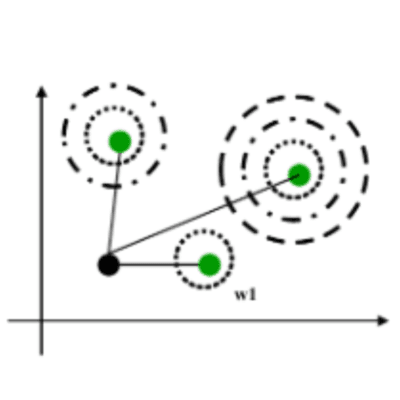
To illustrate, a bit of background as to what happens to data points for modelling geological features, before fitting them with RBFs: they are assigned an attribute that either assigns a distance value, or an indicator value. In either case, the points with a zero value are on the boundary to be modelled, positive values are on one side of that boundary, negative values on the other. Fitting an RBF then operates very similarly to Kriging in estimating values for points that are not in the data set. That is, it estimates for each point how far that point is from the boundary to be modelled, i.e., it assigns an estimated distance and is the definition of an SDF (also see https://en.wikipedia.org/wiki/Signed_distance_function).
Modelling with SDFs
SDFs contain a whole variety of different functions that can be used for this purpose. The most simple and basic one is a (signed) distance from a point or line. In those instances, you cannot really talk about a signed distance as they just return the distance to the point or polyline. Things become slightly different when the points and lines are part of a surface, or in case of a polyline when it is closed, but I’ll leave that to the reader or check online. A great resource is the work done by Inigo Quilez who builds entire 3D models using SDFs (https://iquilezles.org/articles/distfunctions2d/)
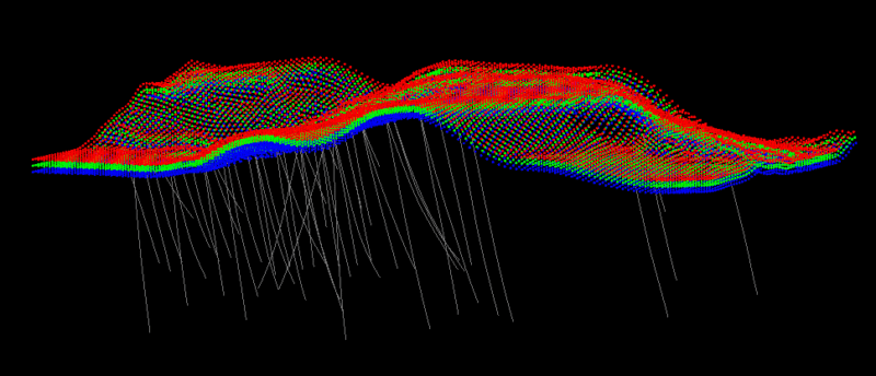
In the case where we have existing surfaces, we can really talk about an SDF. For other data, where multiple points make up a surface such as point clouds from laser scanners, a direct distance estimate does not suffice and neighbouring points need to be used to estimate the SDF. RBFs cannot be directly applied in this case as there are no ‘inside’ and ‘outside’ points. So, a first step is to add so-called “off-surface” points. These are points indicating the sign and are estimated from the surface points. For RBFs there is no need to have these off-surface points at every point of the point cloud and optimizations can be used to estimate how many are needed, but without them the RBF does not work as all the contact points are at zero distance so all points in space not part of the data set will also be estimated to be at zero distance.
Using an SDF is implicit modelling
Hopefully by now, you start to realize that Implicit Modelling is actually a way to estimate distances from a boundary. Now you might ask: “How does that work for grade data, or other numeric data?”. This is a valid question that doesn’t really change the idea described above. For the answer consider you are trying to model a grade shell. This shell is created by using a cut-off grade, let’s say 5 g/t of some mineral. To create the boundary at 5 g/t we can apply a threshold, or better, apply a constant subtraction to all values, meaning all values below 5 g/t will become negative, all values above 5 g/t stay positive. This is a bit like indicator modelling, but you should also see the similarity with the SDFs we mentioned for modelling domains from categorical data as we are not changing the values to indicators.
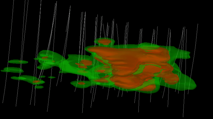
There is one more thing to consider though. In normal life, we understand the concept of distance, e.g., how 1cm is defined, or 1 meter and how far that is from our boundary. For numeric data, this is not as straightforward. We cannot say, at 1 meter from the boundary the grade will be 3 g/t. The lower or higher grade away from the boundary is usually highly non-linear and mostly not constant around all areas of our cut-off. That is where the similarity to our SDF’s ends, and is why a slightly different type of functions is needed for that. However, it can generally be stated that methods used for numeric interpolation and estimation can also be used for modelling boundaries, but methods used to estimate boundaries cannot always be used to estimate numeric values like grades.
Why does it all matter?
Why did we mention all this stuff above you might ask? What’s the point? That is what we will get to now. RBFs have served a great purpose in geological modelling, but its innovation seems to have stopped without further developments in the last 20+ years. However, in those 20+ years developments in other areas have not been idle. This has led to a whole set of algorithms optimized for similar problems that are generally branded under Machine Learning (ML). We won’t go into that too much here as it is part of another blog post. We just want to highlight how ML has resulted in other SDFs specifically focused towards the issue of estimating boundaries from categorical data.
Great speed increase through clever math
No need to worry, we will not go into the math here. We just want to highlight a principle that has helped create enormously fast methods mentioned before.
Typically, signed data points are created from the drilling data although other ways are possible as well. For now, just consider using drilling data to generate many points inside the unit and many points outside. Many of these points are increasingly far away from the boundary that we want to model. This in turn means that many of them are actually redundant.
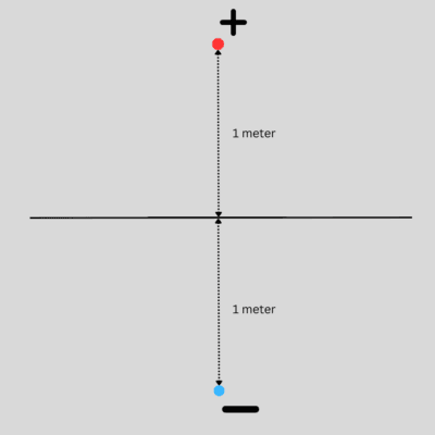
To illustrate, let’s consider a plane, which in a 2D projection becomes a line. If we have a point 1m from this on one side and one point 1m away on the other side. It is easy to see where the point on the boundary will be: exactly in the middle between the two points (assuming of course they are exactly mirrored). If we then add another set of points, 5m away on either side, will they help to know where the point on the boundary is? Not really, as the original two points already defined where the boundary is, so these additional points are actually redundant.
Application from Machine Learning
It is exactly this principle that has let to such incredible speeds observed in ML. Not only in the fitting process as in RBFs, which is called training in ML, but also in the evaluations afterwards. This speed up is only possible by rethinking the modelling process by using SDFs instead of implicit modelling or RBFs. The distance values themselves have a lot of intrinsic value, that when used properly, can greatly speed up the modelling process.
Benefits of Signed Distance Functions
What we hoped to achieve in this article was to have readers rethink what modelling actually does. From this new perspective, lots of new possibilities become apparent. We already mentioned that the processing speeds can be enormously improved. In some of our tests we compared an already very fast RBF interpolation with an ML classification method. The latter uses the knowledge from above about redundant points. In this test, the ML classification was about 100x faster.
If we compare the classification function with a regression method from ML, the speed up is still about 10x.
But speed is only one part. The other is the enormous flexibility it brings by thinking in distances. As mentioned before, to turn a numeric interpolation problem into a signed distance equivalent, we can apply a threshold. This way we can shift where the boundary, in this case a shell, is generated. The reverse can also be applied, by changing the values locally, we can determine where the boundary is located.
To illustrate, we take the plane example from above again. Let’s again assume we have points but this time, not equidistance apart. In this case, the distance of the positive point to the original boundary is halved (0.5), whereas the negative points remains the same (-1.0). Now, the boundary will no longer be in its original position, but roughly at (-1.0 + 0.5) / 2 = -0.25 from that previous location. Press ‘Play’ on the movie to see this illustrated if it does not start automatically.
The flexibility of SDFs
The interesting part now is that when using a function to define the boundary, we don’t actually need to move points. We just have to adjust the value that the function returns. To create a shell, the function is used to evaluate where it returns zero distance as that is where the boundary is located. So, instead of moving a point, we can add a threshold. In the illustration above, this means that to move the original plane to its new location the function just needs to return the original value minus 0.25. If we were to move the plane in the opposite direction by an equal amount, we would add 0.25 to the original value of the function without making any changes to the data!
The key point to remember here is that the value returned by the SDF determines where the boundary is generated.
A simple SDF example: topography
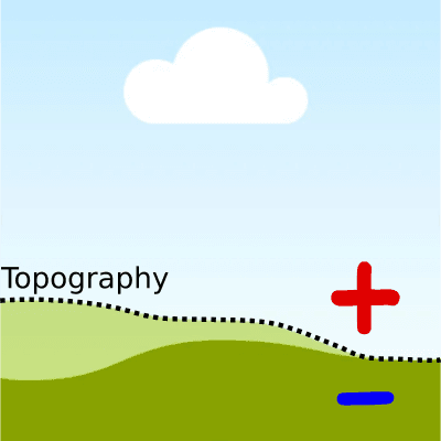
Let’s take a step further now. Instead of a plane and two points we create a very simple function that returns the elevation (the Z-value). Like in previous examples, if the elevation is negative (underground) the function returns a negative value, above the ground it returns a positive value. Now, imagine the elevation is relative to topography. Above the topography everything is positive, below negative. Topography typically is not flat. Not even in my home country, the Netherlands.
For every point we assume to know the topography and we use it as a threshold to the returned elevation. This way at the topography the function always returns zero. We then have a signed distance function that describes the topography.
Extended SDF example: locally modified topography
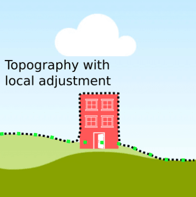
Just like we introduced the topography in our function to return the elevation, we can make further ‘adjustments’. For example, just imagine we are planning a high-rise building on the topography. To model both we can locally adjust the function output to included both the topography AND the high-rise building. Intuitively, this is what you would do yourselves as well. To survey, you would take the topography elevation and add the height of the building to it, only where it exists.
So, now the function, where the high-rise is defined, returns not zero at the topography, but at the top of the high-rise. As you might realize, this is very similar to the way Boolean operations work.
Implicit modelling without triangles
If you grasped this bit, you have just made a huge leap forward in the understanding that has led to a great break-through in 3D graphics in general as all new graphics cards now come with dedicated abilities for real-time ray tracing: a way to draw objects without creating triangulated surfaces.

Final piece of the puzzle: combining SDFs
Now, our final piece of the puzzle: combining functions. Typical SDFs are continuous functions. This means that they cannot cope with hard boundaries or steps easily. This mainly applies to functions being fitted to data, such as RBFs or ML functions. But, as we just demonstrated, a function can be modified, either globally, or locally. Up until now, we have only described how fixed thresholds can be used to change values, but these thresholds could also come from other functions. To illustrate this, consider a simple fault defined by a plane. We can use this plane to split our topography function. On one side of the fault plane, we leave the topography function intact, but on the other side we ignore it. On the other side, we have a different topography function. The combination of the two (three, if we take the fault plane into account as well) now makes up our new topography, still without actually creating a triangulated surface! Likewise, we could draw some polylines or points and adjust our topography SDF based on these manual edits.
As you can see, building models then becomes an exercise in adjusting function values, either globally or locally without committing to building a full model at every step.
Inspirations on SDF and implicit modelling
These concepts have formed the basis of the new modelling framework in GEOREKA since version 4. The principles and ideas mentioned in this article are developed from a plural of sources as part of our research in Horizon 2020 project ROBOMINERS. We specifically highlight 2 sources that have been fundamental to this work: Jun Cowan’s article on wireframe-free modelling (2011: Cowan, E.J., Spragg, K.J. and Everitt, M.R., Wireframe-free Geological Modelling – An Oxymoron or a Value Proposition?, AusIMM Publication Series No 8/2011, 247–259) and Inigo Quilez for his ground-breaking work on the use of SDFs

